
Essentials of Backpropagation in Fully-Connected Feedforward Multilayer Percepetrons
Published:
For the first blog post, I think it is fitting to start with some fundamental topic. Hence, I decided to start with a fundamental topic for mahcine-learning: backpropagation. This is a fundametal mechanism that is widely used in many modern and state-of-the-art methods and deep-learning architectures. So, it is kind of important ![]() . This short view into backpropagation will go over how the mechanism works in simple Fully-Connected Feedforward Multilayer Percepetrons. Even though it remains in how it is appliyed, probably, in a future blog post, I will tackle more complex arquitectures.
. This short view into backpropagation will go over how the mechanism works in simple Fully-Connected Feedforward Multilayer Percepetrons. Even though it remains in how it is appliyed, probably, in a future blog post, I will tackle more complex arquitectures.
Preliminares - How SGD fits.
A neural network is typically non-linear. Hence, it causes most loss functions to become nonconvex. This fact means that traditional convex optimization solvers (e.g., simplex for LP or Newton-type methods) are not suitable for neural network training due to the non-convexity and massive scale of the problem.
Instead of using the traditional methods, nowadays the FFMPs are trained iteratively using gradient-based optimisers that drive the cost function to a very low value (not necessarily the global minimum). Unlike solvers for convex problems, SGD applied to non-convex objectives (such as neural networks) does not guarantee convergence to the global minimum, though it often converges to a local minimum or saddle point. Furthermore, it is sensitive to the initial parameters (weights and bias).
A recurring problem in machine learning is that large training sets are necessary for good generalisation, but large training sets are also more computationally expensive. If we have a cost function that requires computing something that depends on the size of training data, then as the training data grows to billions so will the cost for a single optimisation iteration. Since its first application1 nearly all deep learning2 is powered by one particular version of gradient descent: (batched) SGD. The insight of (batched) SGD is that the gradient is an expectation. The expectation may be approximately estimated using a small set of samples. Specifically, on each step of the algorithm, we can sample a minibatch of examples \(\mathcal{B} = x_0, \dots x_{m^\prime-1}\) drawn uniformly from the training set. The minibatch size \(m^\prime\) is typically chosen to be a relatively small number of examples, ranging from one to a few hundred. Crucially, \(m^\prime\) is usually held fixed even as the training set size \(m\) grows. We may fit a training set with billions of examples using updates computed on only a hundred.
Preliminares - Gradient Descent
We previously mentioned the core on how SGD is applied. We saw the “stochastic part”, but we are yet to see the “gradient descent part”.
Let us start with a small example network, \(M\), consisting of only 3 units. Figure 1 shows the desired network in the usual pictorial manner. In \(M\), the green circle represents the input neuron, the light blue the hidden layer and the orange neuron the output layer.
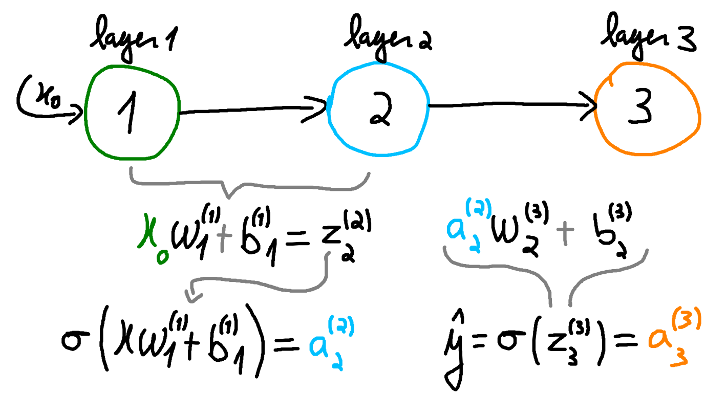
Now let us define some important notation. In Figure 1, the green input unit receives the input \(x_0\) from the user. In the light blue neuron, neuron number 2, it is calculated a weighted input plus a bias from the information that comes from neuron number 1. This originates \(z_2^{(2)} = x_0w_1^{(1)}+b_1^{(1)}\). After, is applied an activation function \(\sigma\), resulting in \(a^{(2)}_2 = \sigma(z_2^{(2)})\). A similar process happens in the orange unit, the output neuron. In this case, the final result, \(a^{(3)}_3\), is typically denoted \(\hat{y}\).
We can think of the arrow connecting the green and light blue neuron carrying \(x_0\) to the light blue neuron. The lgiht blue neuron will try to “extract” information from \(x_0\) with weigthed sum and activation. In this notation, the superscript denotes the layer number and the subscript the order of the weight or bias. As for the subsscript when used in the result of activations, \(a\), and the result of weighted sums, \(z\), it will denote the unit responsible for its calculation. For example, in \(z_2^{(2)}\) we know that this weighted is calculated on layer 2 and is produced in unit 2. This is important for networks with multiple connnections.
We must optimise the weights and biases of all neurons so that the output of the model commonly denoted \(\hat{y}\) is as close to the original value, \(y\), as possible. To define how close \(\hat{y}\) is of \(y\), we use a cost function \(C\). In our pursuit to minimise the error or cost, the learnable parameters (weights and biases) should be adjusted in a manner that reduces this error. To this end, we rely on the gradients of the cost function with respect to each of the learning parameters. These gradients (vector of derivatives) provide information regarding the direction in which parameter updates should be made to effectively diminish the error.
Remember that the derivative of a function \(f\) gives the instantaneous rate of change for all \(x\) in the domain of \(f\). Typically, for a tiny change \(\Delta x\) in \(x\), the change from \(f(x)\) is approximately:
\[\begin{equation}\label{eq:deriv} f(x+\Delta x) - f(x) \approx f^\prime(x) \Delta x \end{equation}\]In other words, \(f^\prime(x)\) gives the expected proportial change in \(f\) per unit of change in \(x\).
Hence, if we calculate the derivative of \(C\) with respect to each weight and bias we will know how their instantaneous rate of change. Using this information, for example, for parameter \(w\), the derivative of \(C\) with respect to \(w\) will tell us how much \(C\) would change for a tiny change in \(w\) in a manner similar to Equation \eqref{eq:deriv}. Since the derivative gives us the rate of steepest ascent, the step that would increase the error the most for tiny change in a parameter, the update is given in the opposite direction (using subtraction), which gives the update rule known as gradient descent.
Looking at Backpropagation
Consider two inputs, \((x_0, y_0)\) and \((x_1, y_1)\). We assume a batch size of one, meaning the parameters are updated after the gradients are calculated for a single example. Let \(C_0 = \tfrac{1}{2}(\hat{y}_0 - y_0)^2\) and let \(\sigma\) be the sigmoid function. For the network in Figure 1, using the chain rule, the partial derivatives required to update \(w^{(3)}_2\) are given in Figure 2.
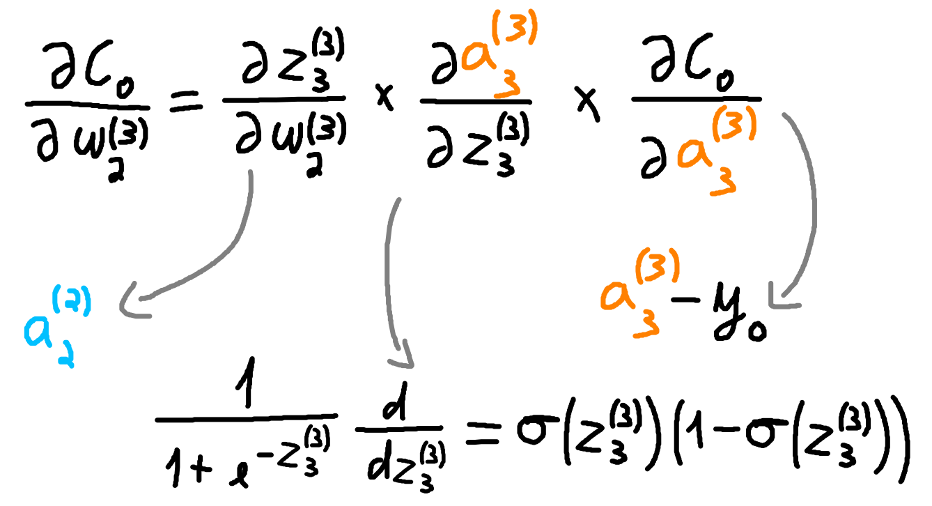
Combining the results from Figure 2, we update \(w^{(3)}_2\) according to Equation \eqref{eq:update-w32}.
\[\begin{equation}\label{eq:update-w32} w^{(3)}_2 = w^{(3)}_2 - \eta \big( a^{(2)}_2 \cdot \sigma(z^{(3)}_3)(1-\sigma(z^{(3)}_3)) \cdot (a^{(3)}_3 - y_0) \big) \end{equation}\]The parameter \(\eta\) represents the learning rate and controls the size of the update step. After updating all weights and biases according to \((x_0,y_0)\), we run the model again and update it based on \((x_1,y_1)\). This completes one epoch. If the batch included both \((x_0,y_0)\) and \((x_1,y_1)\), we would first compute the gradients for both examples, average them, and then perform a single update. Only then would we proceed to the next forward iteration.
Multiple Dependencies
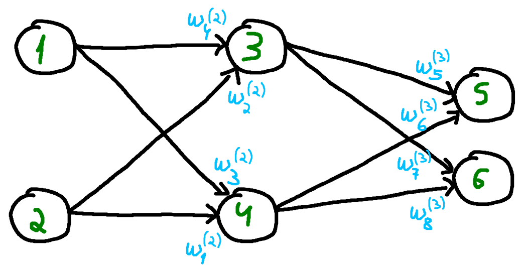
The network used as the example so far only has a single path through which information can travel. This simplifies the computation of the partial derivatives. Consider the network in Figure 3. With multiple paths for information to flow through, the computation of some partial derivatives must take this into account. In Figure 3, the weights are highlighted near the neurons that use them, as well as near the connections they affect. For example, \(w^{(2)}_4\) affects the information that flows from input unit 1 to hidden unit 3.
While the update of the weights in the third layer remains the same as in the previous example, the update of the weights on the second layer change. If the units 1 and 2 were hidden units instead of input units, resulting in a network with two hidden layers, the update of the weights connecting the input to units 1 and 2 would also change. Consider the update of \(w^{(2)}_4\). Since this weight influences the cost function \(C\) from two different paths: the one to unit 5 and the one to unit 6, the chain rule result is slightly different. Figure 4 shows the partial derivatives for this weight update.
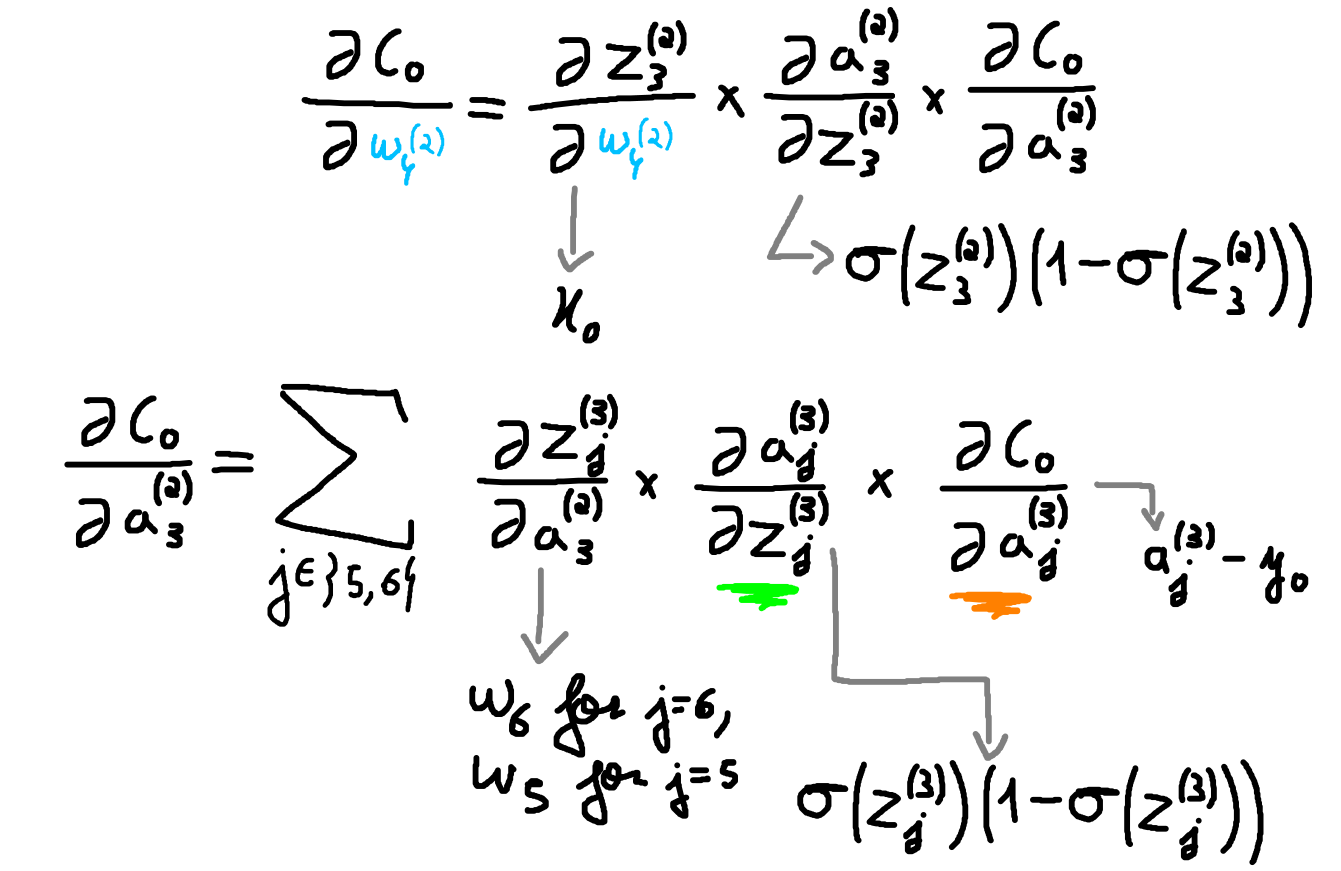
The term highlighted with green and the one highlithed with orange do not need to be calculated since we assume they were backpropagated from the calculations for the update of the weights from layer three. Hence, we can see backpropagation akin to dynamic programming. The concrete update do \(w^{(2)}_4\) is given in Equation \eqref{eq:update24}.
\[\begin{align}\label{eq:update24} \frac{\partial C_0}{\partial a_3^{(2)}} &= \underbrace{\sum_{j \in \{5,6\}} w_j \cdot \sigma \big( z_j^{(3)} \big) \Big(1-\sigma \big( z_j^{(3)}\big)\Big) \cdot (a_j^{(3)} - y_0)}_\tau \tag{3.1} \\ w_4^{(2)} &= w_4^{(2)} - \eta \bigg( x_1 \cdot \sigma \big( z_3^{(2)} \big) \Big(1-\sigma \big( z_3^{(2)}\big)\Big) \cdot \tau \bigg) \tag{3.2} \end{align}\]